Chapter 2 Methodology
Instead of predicting win probability from any game state with one full-stop model, we predict win probability only from kickoff game states10. When the game state is not a kickoff, a series of models first specifies probability distributions for the more granular events that eventually lead to a kickoff and samples are taken from these probability distributions to create a distribution of the possible future game states at the next kickoff. Win probability is then taken to be the mean of the win probability of the distribution of sampled future game states. To implement this a given play is sorted into one of four possible game states: kickoff, extra point, first and ten, and all other game states.
2.1 Modeling Win Probability on Kickoffs and PATs
Model when more than ten minutes remain:
On kickoffs a win probability is modeled using a variation of the trick PFR uses to implement a normal distribution when deriving win probability. For a given game state \(i\) we have:
\(\Delta score_i \sim \mathcal{N}(\hat{\mu}_i,\hat{\sigma}^{2}_i),\)where \(\\ \\ \begin{aligned} \hat{\mu}_i = &\beta_{int} + \beta_\rho\rho_i + \beta_{pos_o}{pos_o}_i + \beta_{de\hspace{-0.1em}f_o}{de\hspace{-0.1em}f_o}_i + \beta_{s_{curr}}s_{curr_i}+ \beta_kk_i + \\ &\beta_{kpos_o}k_ipos_{o_i} + \beta_{k{de\hspace{-0.1em}f_o}}k_i{de\hspace{-0.1em}f_{o_i}} + \beta_{s_{curr}pos_o}s_{curr_i}pos_{o_i} + \beta_{s_{curr}{de\hspace{-0.1em}f_o}}s_{curr_i}{de\hspace{-0.1em}f_{o_i}}\end{aligned}\) and \(\\ \begin{aligned}\hat{\sigma}_i = &\beta_{int} + \beta_{pos_o}{pos_o}_i + \beta_{de\hspace{-0.1em}f_o}{de\hspace{-0.1em}f_o}_i + \beta_{pos_d}{pos_d}_i + \beta_{de\hspace{-0.1em}f_d}{de\hspace{-0.1em}f_d}_i + \beta_{s_{curr}}s_{curr_i} + \beta_{s_{curr_{abs}}}\mid\hspace{-0.2em}{s_{curr_i}}\hspace{-0.2em}\mid + \\ &\beta_tt_i + \beta_{ts}\sqrt{t_i} + \beta_{pos_{qb}}{pos_{qb}}_i + \beta_{de\hspace{-0.1em}f_{qb}}{de\hspace{-0.1em}f_{qb}}_i + \beta_{pos_{qb}s}{pos_{qb}}_is_i + \beta_{de\hspace{-0.1em}f_{qb}s}{de\hspace{-0.1em}f_{qb}}_is_i \end{aligned}\)
Where we define:
\(int =\) Intercept,
\(\rho =\) = Scaled point spread
\(s_{curr} =\) Current score differential
\(s_{curr_{abs}} =\) Absolute value of the current score differential
\(k =\) Team that receives the second half kickoff11
\(t =\) Time remaining in seconds
\(pos_o =\) Offensive DVOA for the team possessing the football
\(pos_d =\) Defensive DVOA for the team possessing the football
\(de\hspace{-0.1em}f_o =\) Offensive DVOA for the team on defense
\(de\hspace{-0.1em}f_d =\) Defensive DVOA for the team on defense
\(pos_{qb} =\) Projected PFF grade for the quarterback of the team with the ball
\(de\hspace{-0.1em}f_{qb} =\) Projected PFF grade for the quarterback of the team on defense
By making the observation that the final score differential is simply \(s_{curr} + \Delta score\) we find:
\(s_{final_i} \sim \mathcal{N}(\hat{\mu}_i + s_{curr_i},\,\hat{\sigma}_i^{2})\) and therefore: \(WinProb_i = P(s_{final_i} > 0) = CDF^{-1}(\frac{\hat{\mu}_i + s_{curr_i}}{\hat{\sigma}_i})\)
Where we define:
\(s_{final} =\) Final score differential
The predictors for \(\mu\) were chosen by performing cross validation in which the most recent season in the training set, 2016, was left out and used as a test set12. Horowitz, Ventura, and Yurko (2018) used a similar method and called it “leave-one-season-out-cross-validation (LOSO CV)”, a term we will modify to leave-most-recent-season-out-cross-validation and brand LMRSO CV. Brier score and log-loss were the primary estimates used to evaluate model performance. The simple linear model used was also tested against a mixed linear model that treated \(k\)—receiving the second half kickoff—as a random effect and utilized an additional intercept as well as random slopes for \(pos_o\) and \(de\hspace{-0.1em}f_o\), but it performed no better than the simple linear model.
Predictors for \(\sigma\) were also chosen using LMRSO CV. The linear model used for \(\sigma\) was also tested against GAMs that were fit with Gamma and Log-Normal distributions using the “gamlss” package developed by Rigby and Stasinopoulos (2005). The “gamlss” package was also used to fit a GAM with an InverseGamma distribution to model \(\sigma^{2}\), but the linear model performed the best by mean-squared error when using LMRSO CV13. This was surprising because the distributions specified when fitting the GAMs seemed more appropriate given the distribution of \(\sigma\) and \(\sigma^{2}\). Ultimately, however, it made the most sense to use the model with the best estimate of \(\sigma\), because only a point estimate of \(\sigma\) is taken as a parameter of the normal distribution.
We also tested a Generalized Linear Mixed Model (GLMM) fit using the “lme4” package and a Generalized Boosted Model (GBM) fitted using Greg Ridgeway’s “gbm” package, used to extend Jerome Friedman’s Gradient Boosted Machine (2001 & 2002). The above model outperforms both the GLMM and the GBM.
Model when ten or fewer minutes remain
The assumption that \(\Delta score\) is normally distributed begins to break down some time around the ten minute mark of the fourth quarter14. Since it is no longer valid to model \(\Delta score\) with a normal distribution, win probability is instead modeled using a GBM that is fit with the following terms.
| Variables |
|---|
| Scaled Point Spread |
| Current Score Differential |
| Square Root of Adjusted Time Left in the Half |
| Offensive DVOA for the Offensive Team |
| Offensive DVOA for the Defensive Team |
| Defensive DVOA for the Offensive Team |
| Defensive DVOA for the Defensive Team |
| Projected QB grade for the Offensive Team |
| Projected QB grade for the Offensive Team |
| Timeouts left for the Offense |
| Timeouts left for the Defense |
Both a Random Forest and the GBM above were considered because of their penchant for fitting data that features predictors with ambiguous interactions, but the GBM was chosen because it performed better in LMRSO CV. Friedman’s Gradient Boosted Machine algorithm (2001 & 2002), implemented in the “gbm” package, works by additively growing a forest of \(n\) decision trees where each tree has a maximum depth \(d\). Trees are added to the forest using gradient descent—each tree must reduce the residual loss as defined by Friedman’s \(K\)-class loss function (2001):
\(-\sum_{k=1}^Ky_klog(p_k(x))\)
In this case the response is binomial so \(K = 2\). A shrinkage parameter \(l\) exists to reduce the learning rate of trees. Lower values generally protect against overfitting but often require more trees to maximize predictive power. The GBM fit above uses parameters \(n = 5000\), \(d = 2\), and \(l = 0.02\).
Overtime model
A GBM fit with the same variables as above but trained only on overtime data is used to determine win probability in overtime situations. This GBM has parameters \(n = 1000\), \(d = 2\), and \(l = 0.02\).
Extra Points
For extra points the process only involves the additional step of sampling \(n\) outcomes for the extra point or two point conversion try15 and passing each resulting game state \(i^*_1, \: i^*_2, \:..., \: i^*_n \sim I^*\) to the model that predicts win probability to find:
\(WinProb_i = \frac{1}{n} \sum_{i^*}^{I^*}WinProb_{i^*}\), where \(WinProb_i^*\) =
\(\:\:\:CDF^{-1}(\frac{\hat{\mu}_{i^*} + s_{curr_{i^*}}}{\hat{\sigma}^{2}_{i^*}})\) if \(t_{i^*} > 600\),
\(\:\:\:GBM_{4th}(i^*)\) if \(0 <t_{i^*} \leq 600\), and
\(\:\:\:GBM_{ot}(i^*)\) if \(t_{i^*} \leq 0\)
2.2 Modeling Win Probability on First and Ten
When the game state features a first and ten we must take \(n\) samples of the pair \((next \: scoring \: event, \: time \: elapsed)\) where, just as in Horowitz, Ventura, and Yurko (2018) the seven possible outcomes for the next scoring event include a touchdown, field goal, or safety for either team and no scoring events before the end of the half. As is done by Horowitz, Ventura and Yurko (2018), the next scoring event is modeled by a multinomial logistic regression, though this work uses the Brian Ripley’s “nnet” package to implement a multinomial logistic regression instead of comparing a set of binary logistic regressions with a chosen baseline event. Modeling end of half, end of game, and overtime situations separately gave the most robust performance by LMRSO CV. The formulas for some of the linear models are the same, but each model was trained only on data within the time window where it would be applied. A multinomial GBM model was also considered. For a given initial game state \(i\) we find the log odds for each possible outcome \(x\) of being the next scoring event \(\delta_x\) as compared to the outcome the algorithm chooses as the baseline16:
\(\begin{aligned}\hat{\delta}_{ix} = &\beta_{intx} + \beta_{xpos_o}{pos_o}_{i} + \beta_{xde\hspace{-0.1em}f_o}{de\hspace{-0.1em}f_o}_i + \beta_{xpos_d}{pos_d}_i + \beta_{xde\hspace{-0.1em}f_d}{de\hspace{-0.1em}f_d}_i + \beta_{xpos_{st}}{pos_{st}}_i + \\ &\beta_{xde\hspace{-0.1em}f_{st}}{de\hspace{-0.1em}f_{st}}_i + \beta_{xt_{adjH}}t_{adjH_i} + \beta_{xc_{score}}c_{score_i} + \beta_{xyrd}yrd_i \\ &\textrm{ if } t_i > 300 \:\: \& \:\: 1800 < t_i \leq 1980, \\ \hat{\delta}_{ix} = &\beta_{xint} + \beta_{xpos_o}{pos_o}_i + \beta_{xde\hspace{-0.1em}f_o}{de\hspace{-0.1em}f_o}_i + \beta_{xpos_d}{pos_d}_i + \beta_{xde\hspace{-0.1em}f_d}{de\hspace{-0.1em}f_d}_i + \beta_{xpos_{st}}{pos_{st}}_i + \\ &\beta_{xde\hspace{-0.1em}f_{st}}{de\hspace{-0.1em}f_{st}}_i + \beta_{xt_{adjH}}t_{adjH_i} + \beta_{xc_{score}}c_{score_i} + \beta_{xyrd}yrd_i \\ &\textrm{ if } 0 < t_i \leq 300, \\ \hat{\delta}_{ix} = &\beta_{xint} + \beta_{xpos_o}{pos_o}_i + \beta_{xde\hspace{-0.1em}f_o}{de\hspace{-0.1em}f_o}_i + \beta_{xpos_d}{pos_d}_i + \beta_{xde\hspace{-0.1em}f_d}{de\hspace{-0.1em}f_d}_i + \beta_{xpos_{st}}{pos_{st}}_i + \\ &\beta_{xde\hspace{-0.1em}f_{st}}{de\hspace{-0.1em}f_{st}}_i + \beta_{xt_{adjH}}t_{adjH_i} + \beta_{xyrd}yrd_i \\ &\textrm{ if } 1800 < t_i \leq 1980, \textrm{and}\\ \hat{\delta}_{ix} = &\beta_{xint} + \beta_{xpos_o}{pos_o}_i + \beta_{xde\hspace{-0.1em}f_o}{de\hspace{-0.1em}f_o}_i + \beta_{xpos_d}{pos_d}_i + \beta_{xde\hspace{-0.1em}f_d}{de\hspace{-0.1em}f_d}_i + \beta_{xpos_{st}}{pos_{st}}_i + \\ &\beta_{xde\hspace{-0.1em}f_{st}}{de\hspace{-0.1em}f_{st}}_i + \beta_{xt_{adjH}}t_{adjH_i} + \beta_{xyrd}yrd_i \\ &\textrm{ if } t_i \leq 0 \end{aligned}\)
Where we define:
\({pos_{st}} =\) Special teams DVOA for the team with the ball
\(de\hspace{-0.1em}f_{st} =\) Special teams DVOA for the defensive team
\(c_{score} =\) Comeback score17
\(yrd =\) Number of yards needed for an offensive touchdown
\(t_{adjH} =\) Timeout adjusted time18 remaining in the half
We don’t need to do any of the work converting the pairwise log odds into a distribution as the “nnet” package does this. We will let \(\hat{\delta}_i\) denote the multinomial distribution of scoring events that we will be sampling from and draw \(n\) samples \(nextScore_{i^*_1}, \: nextScore_{i^*_2},\: ..., \: nextScore_{i^*_n} \sim \mathcal{Multinomial}(\hat{\delta}_i)\). For samples where the next scoring play is a touchdown, the game state is updated to include a draw for the point after that uses the same method outlined in the “Extra Points” sub-heading of 2.1.
Sampling the time elapsed until the next scoring event is a bit trickier19. First, a linear model20 predicts the number of plays, \(\hat{plays}_{i^*}\) for each sample \(i^*\) that take place from the initial game state \(i\) until kickoff for each first and ten game state:
\(\hat{plays}_{i^*} = \beta_{plays}X_{i^*}\)
\(\begin{aligned} \hat{plays}_{i^*} = &\beta_{int} + \beta_{pos_o}{pos_o}_i + \beta_{de\hspace{-0.1em}f_o}{de\hspace{-0.1em}f_o}_i + \beta_{pos_d}{pos_d}_i + \beta_{de\hspace{-0.1em}f_d}{de\hspace{-0.1em}f_d}_i + \beta_{yrd}\sqrt{yrd_i} + \\ &\beta_{c_{score}}c_{score_i} + \beta_{t_{adjH}}\sqrt{t_{adjH_i}} + \beta_{nextScore}nextScore_{i^*} + \beta_{c_{score}yrd}c_{score_i}\sqrt{yrd_i} \end{aligned}\)
The distributions of the number of plays until the next scoring play seems to more closely follow a Log-Normal distribution than a Normal distribution:
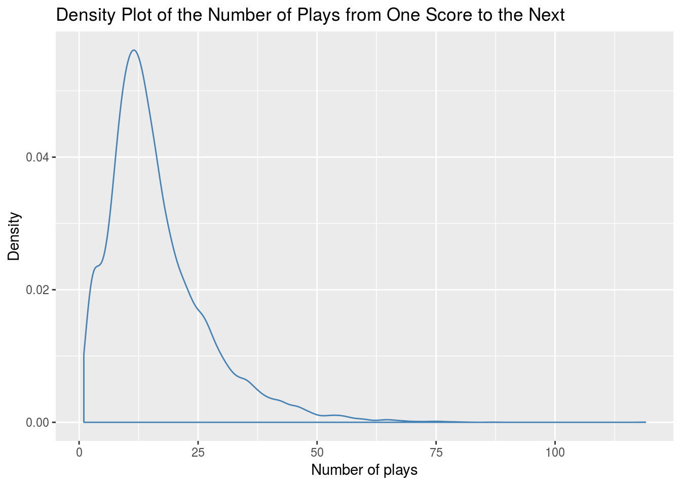
To allow for more accurate sampling of the number of plays from the current game state to the next scoring play the “fitdistrplus” package by Marie-Laure Delignette-Muller is used to choose the parameters of a Log-Normal distribution that fit the data best. \(\sigma^{2}_{plays}\) is set to the variance parameter of the chosen Log-Normal and we sample:
\(log(plays_{i^*}) \sim \mathcal{N}(log(\hat{plays}_{i^*}),\sigma_{plays}^{2})\) so
\(plays_{i^*} = e^{log(plays_{i^*})}\)
To transform each sampled number of plays to time space we split the plays into plays that stopped the clock and plays where the clock continued to run.
\(nStopped_{i^*} \sim \mathcal{Binom}(plays_{i^*}, P_{stopped_{i^*}})\) and
\(nRunning_{i^*} = plays_{i^*} - nStopped_{i^*}\)
Where \(P_{stopped_{i^*}}\) is derived from a GBM detailed in the appendix. Draws that result in fewer than one clock stop are rejected because every scoring play stops the clock.
We next find the total time elapsed. We start by letting
\(K = nStopped_{i^*}\),
\(J = nRunning_{i^*}\),
\(S =\) time elapsed for a play after which the clock stops,
\(R =\) time elapsed for a play after which the clock runs
\(S_{i^*_{1}}, \: S_{i^*_{2}}, \: ... , \: S_{i^*_{K}} \sim \mathcal{N}(\hat{S_i},\sigma_{\epsilon_S}^{2})\) where \(\hat{S_i} = \beta_{int} + \beta_{down}down_i + \beta_{c_{score}}c_{score_i} + \beta_{ydstogo}ydstogo_i + \beta_{c_{score}down}c_{score_i}down_i\)
and
\(R_{i^*_{1}}, \: R_{i^*_{2}}, \: ... , \: R_{i^*_{J}} \sim \mathcal{N}(\hat{R_i},\sigma_{\epsilon_R}^{2})\) where \(\hat{R_i} = \beta_{int} + \beta_{down}down_i + \beta_{c_{score}}c_{score_i} + \beta_{ydstogo}ydstogo_i + \beta_{c_{score}down}c_{score_i}down_i\)
We then find the time elapsed until the next scoring play as:
\(elapsed_{i^*} = \sum_{k=1}^{K}S_k + \sum_{j=1}^{J}R_j\)
Samples from \(\mathcal{N}(\hat{S_i},\sigma_{\epsilon_S}^{2})\) are rejected if they fall outside \([0, 15]\) and samples from \({N}(\hat{R_i},\sigma_{\epsilon_R}^{2})\) are rejected if they fall outside \([15, 50]\) in order to restrict sampled play lengths to a realistic distribution. Additionally, the entire process for sampling a particular value for time elapsed until the next scoring event is repeated if the sample causes an invalid game state21 (i.e. the time elapsed is greater than the amount of time remaining in the half).
Finally, the game states \(i^*_1, \:i^*_2, \:..., \: i^*_n \sim I^*\) are updated in accord with the values that have been sampled and we have:
\(WinProb_i = \frac{1}{n} \sum_{i^*}^{I^*}(WinProb_{i^*}),\) where \(WinProb_{i^*} =\)
\(\: \: \:CDF^{-1}(\frac{\hat{\mu}_{i^*} + s_{curr_{i^*}}}{\sigma^{2}_{i^*}})\) for \(t_{i^*} > 600,\)
\(\: \: \:GBM_{4th}(i^*)\) for \(t_{i^*}\) such that \(0 < t_{i^*} \leq 600\),
\(\: \: \:GBM_{ot}(i^*)\) for \(t_{i^*} \leq 0\)
2.3 Modeling Win Probability in Other Scenarios
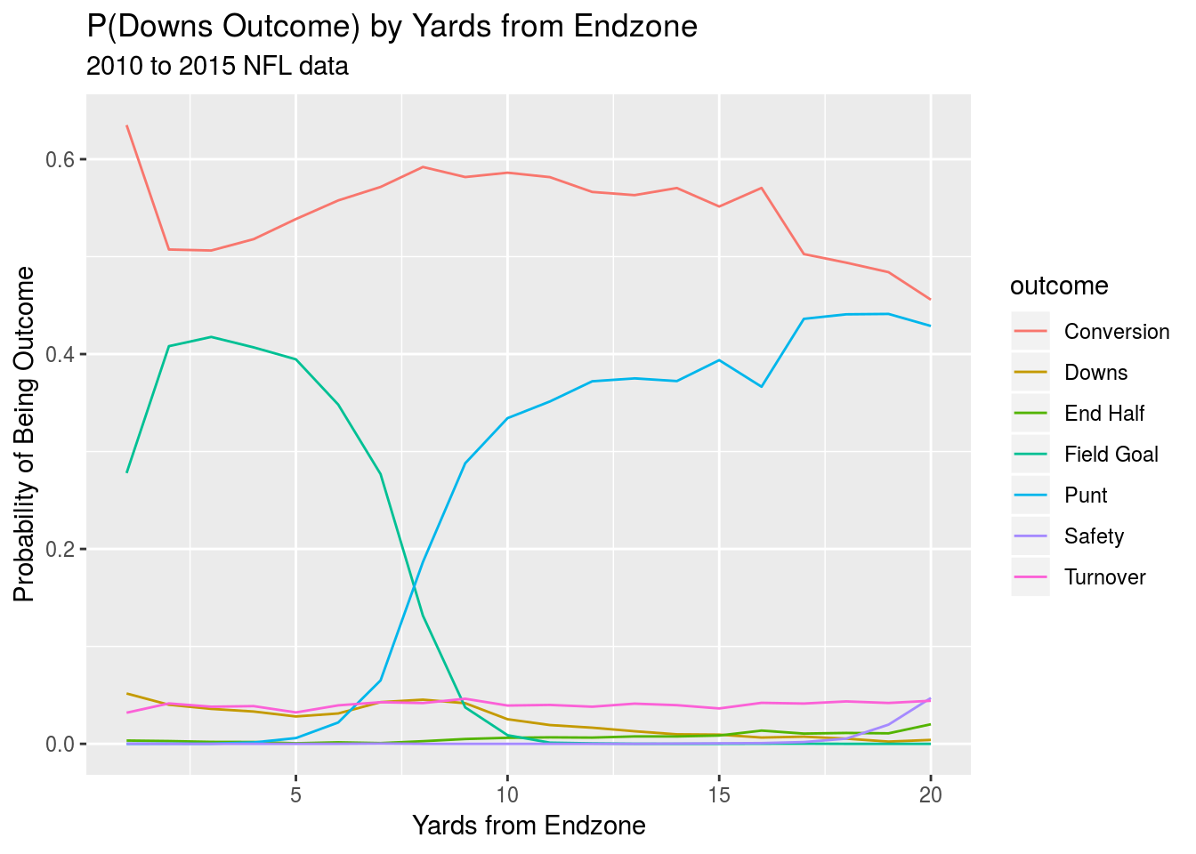
When the game state does not fit any of the scenarios above22, it is first advanced to the next set of downs. To do this we take \(n\) samples of the triple \((outcome \: of \: the \: set \: of \: downs,\: time\: elapsed, scoring \: event)\). We also sample the number of yards downfield the ball will move over the current set of downs for all draws where the current set of downs does not result in a scoring play.
Seven possible outcomes are also defined for a given set of downs: conversion, turnover on downs, end half, field goal attempt, punt, safety, and turnover. As was the case when modeling the next scoring event, end of half, end of game, and overtime game states are modeled separately from other game states. Additionally, separate models were fit for each down because the overall log loss when predicting the outcome for a given set of downs was lower when separate models were fitted for each down during LMRSO CV. End of half, end of game and overtime game states are all modeled with separate GBMs fit using the “gbm” package while all other game states are modeled with a multinomial logistic regression fit using the “nnet” package. The model formulas are listed in the appendix. The models all utilize down, yards to go, DVOA ratings, quarterback grades and a version of yard line that treats each 10 yard increment of the field as a separate group to help the model make better decisions about the likelihood of field goal attempts, punts, and fourth down conversion attempts.
After we have created a distribution \(\delta_i\) of potential outcomes of the set of downs associated with our inital game state \(i\) and sampled \(n\) outcomes \(outcome_{i^*_1}, \: outcome_{i^*_2}, \:..., \:outcome_{i^*_n} \sim \mathcal{Multinomial}(\delta_i)\), we move on to sampling from the distribution of time elapsed. We begin by sampling the number of plays until the next set of downs. This is treated as:
\(\\ \\plays_{i^*} = downstogo_{i^*} + replaysByPenalty_{i^*}\) where \(downstogo_{i^*} = 5 - down_i\) for punts, turnovers on downs, and field goal attempts and \(downstogo_{i^*} \sim \mathcal{M}ultinomial(outcomeDist)\) for conversions, safeties, and turnovers where \(\hspace{-1mm} \begin{aligned} outcomeDist = &(0.349, 0.348, 0.276, 0.027) \textrm{ for conversions, } \\ &(0.363, 0.312, 0.293, 0.032) \textrm{ for turnovers, and } \\ &(0.333, 0.228, 0.272, 0.167) \textrm{ for safeties. } \end{aligned} \\ \\replaysByPenalty_{i^*} \sim \mathcal{B}inom(downstogo_{i^*}, P_{penalty_i})\) where \(P_{penalty_i}\) is taken from a GBM that predicts the probability of a given play being replayed due to penalty. It is listed in the appendix.
\(downstogo_{i^*}\) is set to be \(5 - down_i\) when \(outcome_{i^*}\) is a punt, turnover on downs or field goal attempt because those plays are assumed to happen only on fourth down. The multinomial distributions for conversions, turnovers and safeties simply refer to the probability that an outcome of the given type for a set of downs occurs on a given down. Samples that imply the event happened on a down that has already occurred are rejected. Penalty replays refers to the number of plays until the next set of downs that will be replayed by penalty. To translate a sampled number of plays into time space we use the same equations and process that was detailed in section 2.2.
We next sample whether a given set of downs will result in a scoring play23.
\(score_{i^*} \sim \mathcal{Multinomial}(P_{fg_i}, P_{defTD_i}, P_{noScore_i})\) if \(outcome_{i^*} = field \: goal \: attempt\) and \(score_{i^*} \sim \mathcal{Binom}(P_{score_i} \: | \:outcome_{i^*})\) else
\(P_{score_i} | \:outcome_{i^*}\) is predicted by a GBM for sampled outcomes that are able to result in scores—conversions, field goals, punts and turnovers24. Each GBM was fit using every set of downs that ended with the given outcome. The GBMs are listed in the appendix. For samples where \(score_{i^*} = 1\) and the score is a touchdown, the game state is updated to include a draw for the point after that uses the same method outlined in the Extra Points sub-heading of 2.1. For these samples, as well as any samples where the \(outcome_{i^*}\) is the end of the half, we find that for each updated game_state \(i^*\) the win probability is calculated in the same manner as it was in 2.2:
\(WinProb_{i^*}\) =
\(\:\:\:CDF^{-1}(\frac{\hat{\mu}_{i^*} + s_{curr_{i^*}}}{\hat{\sigma}^{2}_{i^*}})\) for \(t_{i^*} > 600\),
\(\:\:\:GBM_{4th}(i^*)\) for \(t_{i^*}\) such that \(0 < t_{i^*} \leq 600\),
\(\:\:\:GBM_{ot}(i^*)\) for \(t_{i^*} \leq 0\)
For samples where \(score_{i^*} = 0\) we must also sample a value for the number of yards downfield the ball will move over the current set of downs before calculating win probability. For each outcome other than conversions and field goal attempts25, two linear models are defined—one for downs first through third and one for fourth down—that specify a distribution for the number of yards downfield the ball will move for a given game state \(i\). Each linear model is listed in the appendix. The yards moved downfield is modeled separately for each possible outcome because doing so helped most of the linear models meet the assumption of constant residual variance and normally distributed errors26, allowing for easier sampling. The same reasoning is behind separating fourth down data from other data when fitting each model—the residual variance should be lower on fourth down for each outcome type because there is no longer uncertainty about where a punt, field goal attempt, etc. will be taken from. Conversions are a special case and are split into regular conversions and conversions by penalty.
\(P_{penaltyConv_i}\) is defined by a logistic regression that has been trained on all conversion plays. The model only looked at the current down, the yards to go for a first and the interaction between the two variables. Yards moved downfield for conversions by penalty are also modeled with two linear models, one for fourth down and one for any other down. For regular conversions a linear model is specified for each down to better satisfy the linear regression constraints. Field goal attempts also work differently. Field goal attempts that don’t result in a score are classified as either a regular miss or a block.
\(P_{block}\) is modeled using a GBM where the only predictors are yard line27 and down. The change in field position on regular field goal misses is modeled by a linear regression when the down is not fourth. On fourth down the ball is simply moved back 7 yards as is customary on missed field goals. Blocked field goals require the same protocol for determing change in field position as other possible outcomes. One linear model is used for downs first through third and another for fourth. For a given output \(\Delta\hat{fieldPosition}_{i^*}\) from the model \(m\) that is specified by \(outcome_{i^*}\) we take a sample:
Samples drawn are rejected if they result in an invalid or illogical game state. Examples include first down conversions not by penalty where the draw would cause the game state to be short of the first down marker, a turnover on downs where the draw causes the ball to move past the first down marker, or any draw where the resulting game state features a yard line outside \([1, 99]\).
Once we have samples for the number of yards the ball has moved downfield we can fully update each of the game states for which a scoring outcome was not sampled. Each of these \(m \leq n\) remaining game states \(i^*_1, \: i^*_2, \:..., \:i^*_m \sim I^*\) will then go through the process outlined in 2.2. This will lead to the creation of \(M\) new game states \(j^*_1, \: j^*_2, \:..., \:j^*_M \sim J^* \:| \: i^*\) advanced from each game state \(i^*\) and will result in:
\(WinProb_{i^*} = \frac{1}{M}\sum_{j^*}^{J^*}WinProb_{j^* \: | \: i^*}\), where \(WinProb_{j^* \: | \: i^*}\) =
\(\:\:\:CDF^{-1}(\frac{\hat{\mu}_{j^*\:|\:i^*} \: + \: s_{curr_{j^*\:|\:i^*}}}{\hat{\sigma}^{2}_{j^*\:|\:i^*}})\) for \(t_{j*\:|\:i^*} > 600\),
\(\:\:\:GBM_{4th}(j^*\:|\:i^*)\) for \(t_{j^*\:|\:i^*}\) such that \(0 < t_{j^*\:|\:i^*} \leq 600\),
\(\:\:\:GBM_{ot}(j^*\:|\:i^*)\) for \(t_{j^*\:|\:i^*} \leq 0\)
The resulting \(WinProb_i\) for the initial state \(i\) is then computed by taking averaging the values for of win probability for each game state \(i^*_1, \: i^*_2, \:..., \:i^*_n \sim I^*\):28
2.4 Reasoning Behind Modeling Methodology
This methodology has several benefits. The first is that the impact of some game state descriptors like down, yards to go for a first down, and field position should theoretically be easier to measure on events they directly impact, like the outcome of a given set of downs, than on events they indirectly impact, like the probability of winning the game. Reducing noise around the measurement of the effects of game state descriptors like down, yards to go and yard line should improve model accuracy. Another benefit of our method of modeling win probability is that it allows for a full distribution of EPA to be specified rather than a point estimate. This gives a better estimate of the variance associated with a given game state which should lead to more accurate model predictions. Additionally, giving the model an estimate of the distribution of time that will elapse between the current game state and the next score gives the model an even fuller picture of the game and helps prevent incongruities. Our modeling methodology also makes it easier to update the model piecemeal. If research comes out about the factors that influence the likelihood of converting a given set of downs, it shouldn’t be difficult to incorporate the findings into the multinomial models that handle predicting the outcome of a given set of downs. Our methodology yields many of the benefits of a simulation without having to specify an exhaustive grid of conditional probabilities29.
Each of the models will be described in greater detail later on in the section↩
1 if the team that has the ball will receive the second half kickoff, -1 if the defensive team will receive the second half kickoff, and 0 if the game is already past halftime↩
The most recent season was chosen as the season to leave out because the model will always be tasked with using past results to predict future results in practice, and it seems likely that rule changes and evolving strategy could cause gradual changes in game play over time. If these changes are even somewhat smooth, it will be useful to tune models on data that will differ from the training set in a similar manner to the way the next season’s batch of data will differ from the current season’s.↩
Error for \(\sigma^{2}\) was determined after taking the square root↩
\(\Delta score\) follows the normal distribution longer than we found raw change in score differential to follow the normal distribution. This is likely because of the addition of a model for \(\hat{\mu}\) instead of using a mean of 0.↩
A chart defining situations where a team is classified as going for two is listed in the appendix↩
A conversion in this case↩
The comeback score variable is meant to define the urgency of a comeback situation to help the models that measure time elapsed provide more accurate probability distributions when the game state is being advanced. It is also used in some of the end of game models as a feature that gives an indication of the relationship between score differential and time remaining.↩
The amount of time remaining in the half + 20 secs for every timeout possessed by a team with a comeback score of four or five↩
Except when the next scoring play is sample to be the end of the half in which case time elapsed is just the time remaining in the half↩
It outperformed a GAM assuming a Log-Normal distribution with the same inputs by LMRSO CV↩
If a sample is rejected more than 10 times it is that the game state that will result in the end of the half and was misclassified↩
This will occur on any second, third, or fourth down play, as well as on first downs where there are more or less than ten yards to go↩
All sets of downs where the sampled outcome is a safety are treated as scoring plays↩
Scores on conversions are assumed to be offensive touchdowns and scores on punts and turnovers are assumed to be defensive touchdowns↩
and end of halves where we don’t need to sample this quantity at all↩
The exception to this is when the outcome of the set of downs is a conversion, but rejecting samples that were behind the first down marker alleviated this.↩
Given a missed field goal, the shorter the attempt was, the more likely it was to be blocked↩
This includes the game states for which \(score_{i^*}\) is equal to one and \(WinProb_{i^*}\) was calculated earlier.↩
Though this modeling protocol certainly comes with its fair share of edge cases to account for.↩