A Appendix
A.1 QB Model
A linear model was deemed sufficient for predicting a the PFF grade for a quarterback in a given seasons using past data. For a given quarterback and season combination \(i\), we have:
\(grade_{i} = \beta_{int} + \beta_{1}smoothGrades_i + \beta_{2}draftPick_i + \beta_{3}prevAttempts_i + \epsilon_i\)
where \(smoothGrades_i\) refers to a the weighted average of the grades a quarterback has received in previous seasons with more recent seasons weighted more heavily using a smooth exponential decay function with \(decay = 0.3\). A prior number of attempts of league average quarterback play was added to each grade outputted by the decay function. \(prior = 1500\) was chosen to minimize error through LMRSO CV.
A.2 Two Point Chart
The (very) naive two point decision making models assumes that teams go for two when the score differential is one of the following during the period between the touchdown and point after attempt:
| Two Point Conversion Score Differentials | 19, | 12, | 5, | 4, | 1, | -2, | -9, | -10, | -16, | 17, | -18 |
A.3 GBM for \(P_{stopped}\)
This GBM predicts the probability of the clock stopped on a given play by using the variables listed in the table below. The value for each variable is the value for the variable at the previous kickoff to account for that face that this model has to predict the probability of the clock stopping not just for the current play but also for some number of plays in the future despite being unable to update other information. The model uses the shrinkage parameter \(l = 0.02\), an interactions depth of two and \(1000\) trees.
| Variables |
|---|
| Clock Will Stop |
| Number of Plays Until the Next Scoring Event |
| Timeout Adjusted Time Remaining in the Half |
| The Comeback Score |
A.4 Downs Outcome Formulas
For an initial game state \(i\), when \(t_i > 300\) & !\((1800 < t_i <= 1980)\) a multinomial logistic regression model is fit, mimicking the process used to predict the next scoring event. The log odds \(\delta_ix\) for a given outcome \(x\) as compared to the baseline outcome are modeled by:
\(\delta_ix = \beta_{xint} +\beta_{xpos_{o}}pos_{o_i} + \beta_{xde\hspace{-0.1em}f_{o}}de\hspace{-0.1em}f_{d_i} +\beta_{xpos_{{qb}}}pos_{{qb}_i} + \beta_{xydstogo}ydstogo_i + \beta_{xyrd_{group}}yrd_{group_{i}}\)
Each GBM uses the following variables as well as a shrinkage parameter \(l = 0.02\), an interaction depth of two, and \(1000\) trees. The data on which they are trained is the only difference between the GBMs.
| Variables |
|---|
| Offensive DVOA for the Team with the Ball |
| Defensive DVOA for the Team on Defense |
| Projected QB Grade for the Offensive Team |
| Yards to go for a First Down |
| Score Differential |
| Timeout Adjusted Time Remaining in the Half |
| Yards from the End Zone Bucketed in Ten Yard Increments |
A.5 GBM for \(P_{penaltyReplay}\)
To output the probability of a penalty on a given play the GBM takes in the current down, the outcome of the set of downs and the field position of the offensive team. The shrinkage is given by \(l = 0.005\), the interaction depth is two and the number of trees is 1000.
A.6 GBMs for \(P_{score}\)
The GBM that predicts \(P_{TD}\:| \:Conversion\) also uses a shrinkage parameter \(l = 0.02\), an interaction depth of two, and 1000 trees. It is fit with the following variables:
| Variables |
|---|
| Offensive DVOA for the Team with the Ball |
| Defensive DVOA for the Team on Defense |
| Projected QB Grade for the Offensive Team |
| Yards to go for a First Down |
| Down |
| Yards from the End Zone |
The GBM that predicts \(P_{defTD}\:|\:Turnover\) utilizes a shrinkage parameter \(l = 0.02\), an interaction depth of two and 1000 trees. It is fitted with only three variables—the square root of yards from the end zone for the team punting, the offensive DVOA for the team on offense and the defensive DVOA for the team on defense.
The GBM that predicts \(P_{defTD}\:|\:Punt\) utilizes a shrinkage parameter \(l = 0.005\), an interaction depth of two and 1000 trees. It is fitted with only three variables—the yards from the end zone for the team punting and the special teams DVOAs for both teams.
The GBM that predicts \(P_{Make}\:|\:FG Attempt\) depends only on the square root of yards from the end zone for the team kicking the field goal, as does the GBM that predicts the \(P_{defTD}\:|\:FG Block\). Both have \(l = 0.01\) and \(ntrees = 1000\), though the field goal make GBM uses an interaction depth of one while the field goal block GBM uses an interaction depth of two.
A.7 Linear Models for \(\Delta \: field \: position_{i^*} | outcome_{i^*}\)
Conversion
For first and second down all models for change in field position for conversions have the same formula. A given model \(m\) has formula as follows. A reminder that \(yrds\) is the field position of the offensive team:
\(y_{mi} = \beta_{mint} + \beta_{m1}ydstogo_i + \beta_{m2}\sqrt{yrds_i} + \beta_{m3}pos_{o_i} + \beta_{m4}def_{d_i} + \epsilon_{mi}\)
For third downs the model has formula:
\(y_{i} = \beta_{int} + \beta_{1}ydstogo_i + \beta_{2}\sqrt{yrds_i} + \beta_{3}pos_{qb_i} + \epsilon_i\)
and on fourth downs the model has formula:
\(y_{i} = \beta_{int} + \beta_{1}ydstogo_i + \beta_{2}\sqrt{yrds_i} + \beta_{3}pos_{o_i} + \epsilon_i\)
Conversion by Penalty
The model that handles first through third down has form:
\(y_{i} = \beta_{int} + \beta_{1}ydstogo_i + \beta_{2}\sqrt{yrds_i} + \beta_{3}down_i + \beta_{4}down_iydstogo_i + \epsilon_i\)
The model for fourth downs is:
\(y_{i} = \beta_{int} + \beta_{1}ydstogo_i + \beta_{2}\sqrt{yrds_i} + \epsilon_i\)
Turnover on Downs
The model for first through third down looks like:
\(y_{i} = \beta_{int} + \beta_{1}ydstogo_i + \beta_{2}\sqrt{yrds_i} + \beta_{3}pos_{qb_i} + \beta_{4}t_{adjH} + \beta_{5}t_{adjH}\sqrt{yrds_i} + \epsilon_i\)
The model for fourth downs is much simpler:
\(y_{i} = \beta_{int} + \beta_{1}ydstogo_i + \epsilon_i\)
Punt
The model for first through third down is:
\(y_{i} = \beta_{int} + \beta_{1}ydstogo_i + \beta_{2}\sqrt{yrds_i} + \beta_{3}pos_{st_i} + \beta_{4}def_{st_i} + \epsilon_i\)
The fourth down model is:
\(y_{i} = \beta_{int} + \beta_{1}\sqrt{yrds_i} + \beta_{2}pos_{st_i} + \beta_{3}def_{st_i} + \epsilon_i\)
Turnover
Though the field position change for turnovers is also modeled with separate models for fourth down and first through third down, the model formula is the same for both models (though coefficients are different). For a given model \(m\):
\(y_{mi} = \beta_{int} + \beta_{m1}ydstogo_i + \beta_{m2}\sqrt{yrds_i} + \beta_{m3}pos_{qb_i} + \epsilon_{mi}\)
Field Goal
The model for change in field position on missed field goals given the current down not being fourth is:
\(y_{i} = \beta_{int} + \beta_{1}ydstogo_i + \beta_{2}def_{d_i} + \beta_{3}down_i + \beta_{4}ydstogo_idown_i + \epsilon_{i}\)
For blocked field goals the model for change in field position on downs one through three is:
\(y_{i} = \beta_{int} + \beta_{1}ydstogo_i + \beta_{2}def_{d_i} + \beta_{3}\sqrt{yrds_i} + \epsilon_{i}\)
On fourth down the model is:
\(y_{i} = \beta_{int} + \beta_{1}\sqrt{yrds_i} + \epsilon_{i}\)
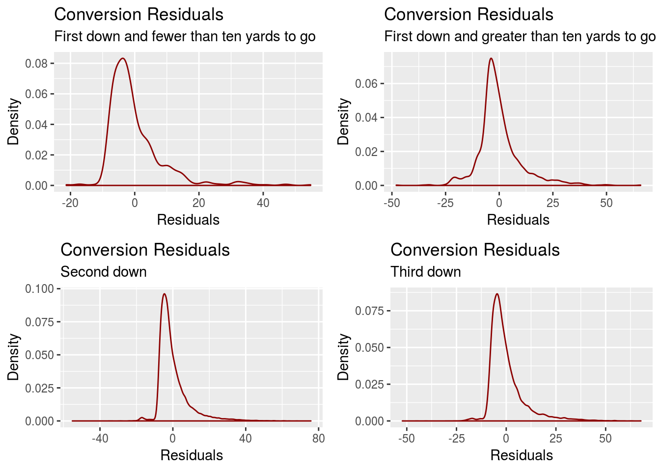
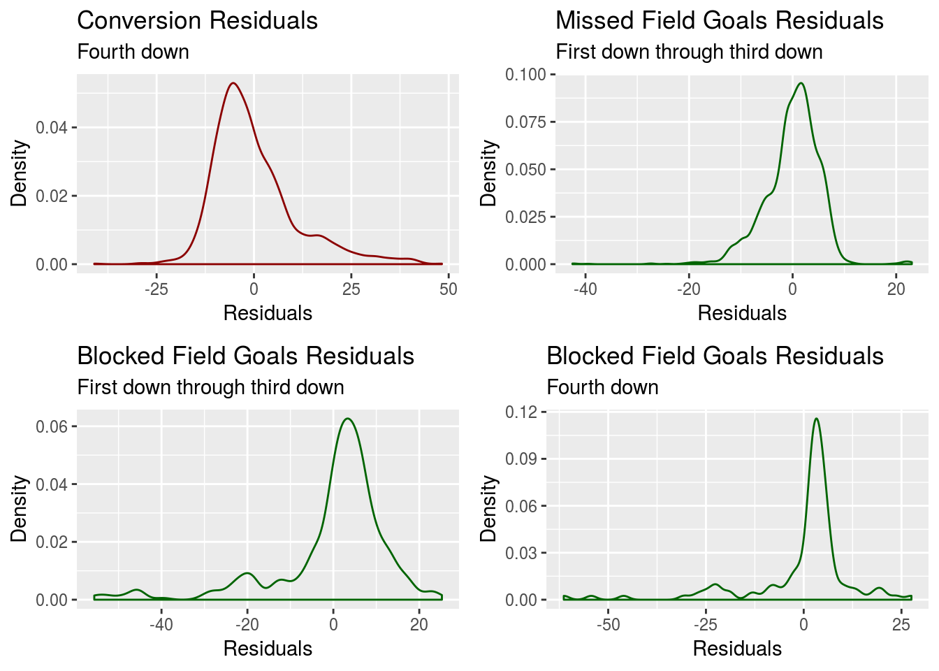
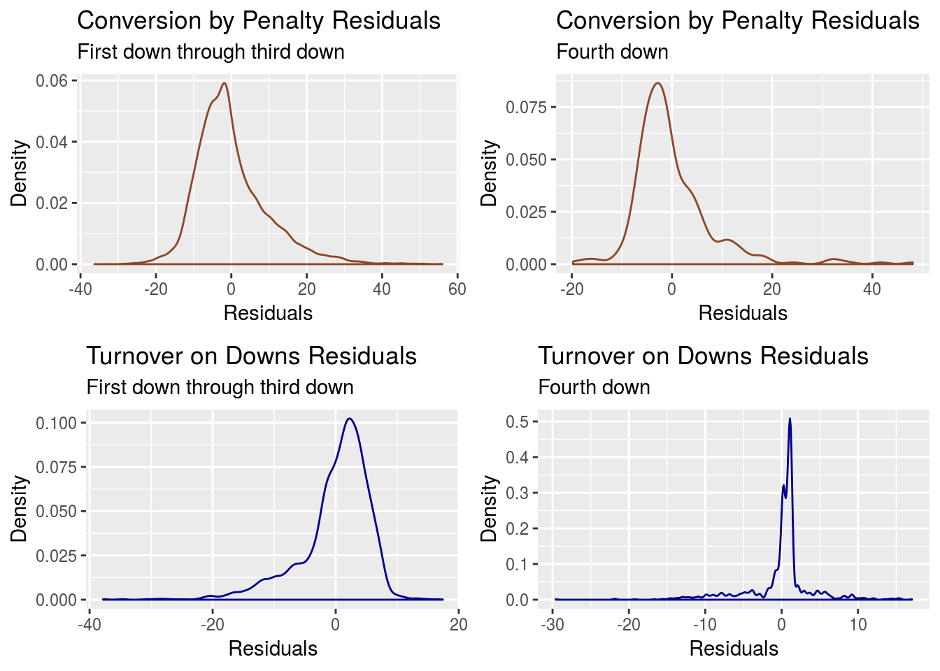
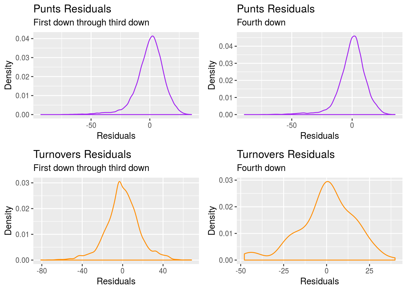
A.8 Residual Plots for \(\Delta \: field \: position_{i^*} | outcome_{i^*}\)
A reminder that when sampling from \(\mathcal N(\Delta \: field \: position, \sigma^{2}_{\epsilon})\), values that would lead to incoherent game stats are rejected. This fixes issues with the lack of normality for the residual distributions of \(\Delta \: field \: position_{i^*}\) when the sampled outcome \(outcome_{i^*}\) is either a conversion or a turnover on downs.